Dynamic Light Scattering (DLS)
According to the semiclassical light scattering theory when light impinges on matter, the electric field of the light induces an oscillatingĀpolarization of electrons in the molecules. The molecules then serve as secondary source of light and subsequently radiate (scatter) light. The frequency shifts, the angular distribution, the polarization, and the intensity of the scatter light are determined by the size, shape and molecular interactions in the scattering material.
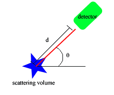
The set up of a dynamic light scattering experiment is shown above
Light intensity is I(t) at time t
At the time t + t, which is a very small time later than t, the diffusing particles will have new positions and the intensity at the detector will have a value I(t+t)
The detector saves the values for I(t + t) at numerous (80 in the N4 Plus DLS) times (Actually, the autocorrelator automatically calculates the function instead of the discrete intensities)
Shown below is an example of a light scattering experiment. -A- shows time zero. -B- is after a short time. -C- is after a longer time period.
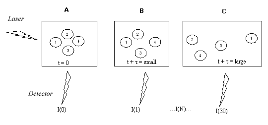 I(t+t) correlates with I(t), the closer the measurement is to time zero, the more similar I(t+t) is to I(t) since the particles have not had much time to move (Panel B):
As time goes on there is no more similarity between the starting state and the current state (Panel C) - the measured intensities do no correlate anymore to the beginning one. This happens faster if the particles are smaller since smaller particles move faster. One needs a method for quantifying how fast the correlation takes to break down between the starting measurement and one a short time later.
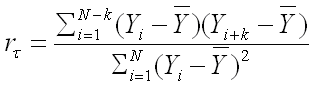
The function used to calculate this correlation is the autocorrelation function it describes how a given measurement relates to itself in a time dependent manner:
At time zero, r = 1 i.e. there is a 100% autocorrelation. As time progresses, the autocorrelation diminishes reaching zero as there is no more similarity between starting and ending states.
Try this: Show r = 1 when t=0!
The decay of the autocorrelation is described by an exponential decay function G(t) which relates the autocorrelation to the diffusion coefficient D and the measurement vector K:
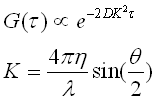
n = refractive index of the solution (1.33 for water)
l = wavelength of the laser (632.8 nm in the N4)
q = angle of scattering measurement (Your choice: 15.2, 21.1, 31.1, 41.9, 51.8, 90 degrees)
Try this: Use Excel to plot the function G(t) for various D and K!
By fitting the points of autocorrelation to the function G(t), the diffusion coefficient can be measured and related to the equivalent sphere of diameter d using the Stokes - Einstein equation:
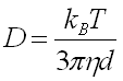
n = diluent viscosity (water = 8.94*10-4 kg/(ms)
T = Temperature (K) (room temp = 298 K)
D = diffusion coefficient (in m2/s)
kB = Boltzmann constant (1.3807*10-23 J/K)
d = sphere diameter (m)
For proteins:
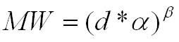
d = sphere diameter in nm
a = correction factor 1 = 1.68
b = correction factor 2 = 2.3398
MW = mol. weight in kDa
Try this: many instruments can only measure 3 to 3000 nm particles - what is the approximate equivalent range of spherical protein molecular weights?